Data Analysis: Cell frequency analysis#
In this vignette we showcase FACSPy functionality in order to get a quick overview over the sample metrics.
This will include cell counts and gate frequencies.
First, we import the necessary library and load the dataset we created in the previous vignette.
[1]:
import warnings
warnings.filterwarnings(
    action='ignore',
    category=FutureWarning
)
[2]:
import FACSPy as fp
[3]:
dataset = fp.read_dataset(input_dir = "../../Tutorials/mouse_lineages",
                          file_name = "raw_dataset")
dataset
[3]:
AnnData object with n_obs × n_vars = 3212862 × 20
    obs: 'staining', 'sample_ID', 'file_name', 'organ', 'genotype', 'sex', 'experiment', 'age'
    var: 'pns', 'png', 'pne', 'pnr', 'type', 'pnn', 'cofactors'
    uns: 'metadata', 'panel', 'workspace', 'gating_cols', 'dataset_status_hash', 'cofactors', 'raw_cofactors', 'settings', 'pca_CD45+_transformed', 'pca_CD45+_logicle'
    obsm: 'X_pca_CD45+_logicle', 'X_pca_CD45+_transformed', 'gating'
    varm: 'pca_CD45+_logicle', 'pca_CD45+_transformed'
    layers: 'compensated', 'logicle', 'transformed'
Since we do not need the unstained samples anymore, we will exclude them.
Here, we subset the dataset and will synchronize the metadata in the .uns slot.
[4]:
dataset = dataset[dataset.obs["staining"] != "unstained",:].copy()
fp.sync.synchronize_dataset(dataset)
Found modified subsets: ['adata_obs_names', 'adata_sample_ids']
        ... synchronizing metadata object to contain sample_IDs of the dataset
C:\Users\tarik\anaconda3\envs\FACSPypeline\lib\site-packages\FACSPy\exceptions\_exceptions.py:12: UserWarning: It was detected that the dataset was modified.Please make sure that the performed analyses are still valid. Note that if you removed whole samples, mfi/fop calculations will not be affected.
  warnings.warn(message, UserWarning)
C:\Users\tarik\anaconda3\envs\FACSPypeline\lib\site-packages\FACSPy\synchronization\_synchronize.py:106: DataModificationWarning: 'It was detected that the dataset was modified.Please make sure that the performed analyses are still valid. Note that if you removed whole samples, mfi/fop calculations will not be affected.'
  warnings.warn('', DataModificationWarning)
[5]:
dataset.uns["metadata"].to_df()
[5]:
| sample_ID | file_name | organ | genotype | sex | experiment | age | staining | |
|---|---|---|---|---|---|---|---|---|
| 10 | 11 | 21112023_lineage_BM_M10_014.fcs | BM | neg | f | 2 | 95 | stained |
| 11 | 12 | 21112023_lineage_BM_M11_015.fcs | BM | pos | m | 2 | 95 | stained |
| 12 | 13 | 21112023_lineage_BM_M12_016.fcs | BM | pos | m | 2 | 95 | stained |
| 13 | 14 | 21112023_lineage_BM_M7_011.fcs | BM | neg | f | 2 | 95 | stained |
| 14 | 15 | 21112023_lineage_BM_M8_012.fcs | BM | pos | f | 2 | 95 | stained |
| 15 | 16 | 21112023_lineage_BM_M9_013.fcs | BM | neg | f | 2 | 95 | stained |
| 18 | 19 | 22112023_lineage_BM_M13_011.fcs | BM | pos | m | 3 | 96 | stained |
| 19 | 20 | 22112023_lineage_BM_M14_012.fcs | BM | pos | m | 3 | 96 | stained |
| 20 | 21 | 22112023_lineage_BM_M15_013.fcs | BM | pos | m | 3 | 96 | stained |
| 21 | 22 | 22112023_lineage_BM_M16_014.fcs | BM | neg | f | 3 | 96 | stained |
| 22 | 23 | 22112023_lineage_BM_M17_015.fcs | BM | neg | f | 3 | 96 | stained |
| 23 | 24 | 22112023_lineage_BM_M18_016.fcs | BM | neg | m | 3 | 96 | stained |
| 2 | 3 | 20112023_lineage_BM_M1_038.fcs | BM | pos | f | 1 | 95 | stained |
| 3 | 4 | 20112023_lineage_BM_M2_039.fcs | BM | neg | f | 1 | 95 | stained |
| 4 | 5 | 20112023_lineage_BM_M3_040.fcs | BM | pos | f | 1 | 95 | stained |
| 5 | 6 | 20112023_lineage_BM_M4_041.fcs | BM | pos | m | 1 | 95 | stained |
| 6 | 7 | 20112023_lineage_BM_M5_042.fcs | BM | neg | m | 1 | 95 | stained |
| 7 | 8 | 20112023_lineage_BM_M6_043.fcs | BM | neg | m | 1 | 95 | stained |
Cell Count analysis#
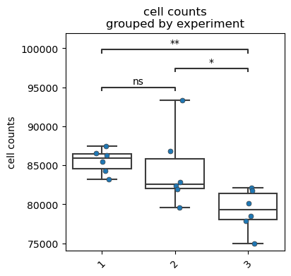
We first plot the raw cell counts using the fp.pl.cell_counts(). As with every visualization plot, we pass a gate to specify which population to analyze. Note the vignette ‘FACSPy gate handling’ for further information on how to handle gates.
You can specify a full gate path, a partial gate path or just the final population.
[6]:
fp.pl.cell_counts(dataset,
                  gate = "CD45+",
                  groupby = "experiment",
                  figsize = (4,4))
No artists with labels found to put in legend. Note that artists whose label start with an underscore are ignored when legend() is called with no argument.
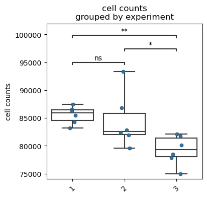
[7]:
fp.pl.cell_counts(dataset,
                  gate = 'root/cells/singlets/live/CD45+',
                  groupby = "experiment",
                  figsize = (4,4))
No artists with labels found to put in legend. Note that artists whose label start with an underscore are ignored when legend() is called with no argument.
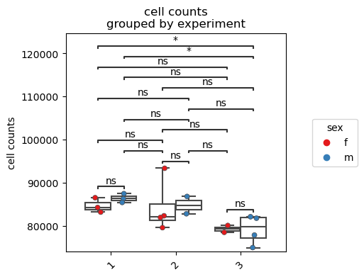
Further customization of the plot is possible. Here, we use the splitby parameter in order to visualize potential differences between the sexes.
[8]:
fp.pl.cell_counts(dataset,
                  gate = "CD45+",
                  groupby = "experiment",
                  splitby = "sex",
                  figsize = (4,4))
Gate frequency analysis#
One of the most common analysis in cytometry is the quantification of gates. We first calculate the gate frequencies using the fp.tl.gate_frequencies() function.
[9]:
fp.tl.gate_frequencies(dataset)
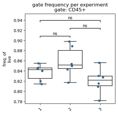
For visualization, we use the fp.pl.gate_frequency() function. We specify the gate as well as the parent we want to visualize.
For the freq_of parameter, valid inputs are ‘parent’, ‘grandparent’, ‘all’ or a gate.
[10]:
fp.pl.gate_frequency(dataset,
                     gate = "CD45+",
                     freq_of = "parent",
                     groupby = "experiment",
                     figsize = (4,4))
No artists with labels found to put in legend. Note that artists whose label start with an underscore are ignored when legend() is called with no argument.
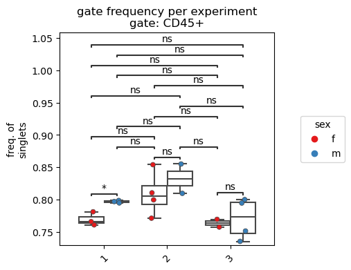
Similar to the cell count plot, we can further customize the data graph.
[11]:
fp.pl.gate_frequency(dataset,
                     gate = "CD45+",
                     groupby = "experiment",
                     splitby = "sex",
                     freq_of = "grandparent",
                     figsize = (4,4))
Save the dataset#
Since we performed the gate frequency analysis, we save the dataset.
[12]:
fp.save_dataset(dataset,
                output_dir = "../../Tutorials/mouse_lineages/",
                file_name = "raw_dataset_stained",
                overwrite = True)
File saved successfully