FACSPy.pl.biax#
- FACSPy.pl.biax(adata, gate, layer, x_channel, y_channel, sample_identifier=None, color='density', add_cofactor=False, x_scale=None, y_scale=None, color_scale='linear', cmap=None, vmin=None, vmax=None, title=None, figsize=(4, 4), return_dataframe=False, return_fig=False, ax=None, show=True, save=None, **kwargs)#
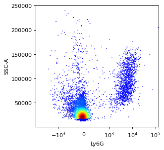
Plot for normal biaxial representation of cytometry data.
Color the plot using annotations of observations (.obs) or expression of markers. Axes are customizable to log, biex or linear scale.
- Parameters:
adata (
AnnData) – The anndata object of shape n_obs x n_vars where rows correspond to cells and columns to the channelsgate (
str) – The gate to be analyzed, called by the population name. This parameter has a default stored in fp.settings, but can be superseded by the user.layer (
str) – The layer corresponding to the data matrix. Similar to the gate parameter, it has a default stored in fp.settings which can be overwritten by user input.x_channel (
str) – The channel that is plotted on the x axis.y_channel (
str) – The channel that is plotted on the y axissample_identifier (
Optional[str]) – Controls the data that are extracted. Defaults to None. If set, has to be one of the sample_IDs or the file_names.color (
Optional[Union`[:py:class:`str,Literal['density']]]) – The parameter that controls the coloring of the plot. Can be set to categorical variables from the .obs slot or continuous variables corresponding to channels. Default is set to ‘density’, which calculates the point density in the plot.add_cofactor (
Union[Literal['x','y','both'],bool]) – if set, adds the cofactor as a line to the plot for visualization. if x, sets the cofactor for the x-axis, if y, sets the cofactor for the y-axis, if both, sets both axis cofactorsx_scale (
Optional[Literal['biex','log','linear']]) – sets the scale for the x axis. Has to be one of biex, log, linear. The value biex gets converted to symlog internallyy_scale (
Optional[Literal['biex','log','linear']]) – sets the scale for the y axis. Has to be one of biex, log, linear. The value biex gets converted to symlog internallycolor_scale (
Literal['biex','log','linear']) – sets the scale for the colorbar. Has to be one of biex, log, linear.cmap (
Optional[str]) – Sets the colormap for plotting. Can be continuous or categorical, depending on the input data. When set, both seaborns palette and cmap parameters will use this valuevmin (
Optional[Union`[:py:class:`float,int]]) – minimum value to plot in the color vectorvmax (
Optional[Union`[:py:class:`float,int]]) – maximum value to plot in the color vectortitle (
Optional[str]) – sets the figure title. Optionalfigsize (
tuple[float,float]) – Contains the dimensions of the final figure as a tuple of two ints or floats.return_dataframe (
bool) – If set to True, returns the raw data that are used for plotting as a dataframe.return_fig (
bool) – If set to True, the figure is returned.ax (
Optional[Axes]) – AAxescreated from matplotlib to plot into.show (
bool) – Whether to show the figure. Defaults to True.save (
Optional[str]) – Expects a file path including the file name. Saves the figure to the indicated path. Defaults to None.kwargs – keyword arguments that will ultimately passed to sns.scatterplot().
- Return type:
Optional[Figure,Axes,DataFrame]]- Returns:
If show==False a
AxesIf return_fig==True a
FigureIf return_dataframe==True a
DataFramecontaining the data used for plotting
Examples
import FACSPy as fp

dataset = fp.mouse_lineages()

fp.pl.biax(
    dataset,
    gate = "CD45+",
    layer = "compensated",
    x_channel = "Ly6G",
    y_channel = "SSC-A",
    color = "density",
    x_scale = "biex",
    y_scale = "linear"
)