Data analysis: Fluorescence intensity and Frequency of Parents#
In this vignette we will cover how to calculate MFIs and FOPs and visualize them.
We will first import necessary libraries and read our dataset we created in earlier vignettes.
[1]:
import warnings
warnings.filterwarnings(
    action='ignore',
    category=FutureWarning
)
[2]:
import FACSPy as fp
[3]:
dataset = fp.read_dataset(input_dir = "../../Tutorials/mouse_lineages/",
                          file_name = "raw_dataset_stained")
dataset
[3]:
AnnData object with n_obs × n_vars = 2450306 × 20
    obs: 'staining', 'sample_ID', 'file_name', 'organ', 'genotype', 'sex', 'experiment', 'age'
    var: 'pns', 'png', 'pne', 'pnr', 'type', 'pnn', 'cofactors'
    uns: 'metadata', 'panel', 'workspace', 'gating_cols', 'dataset_status_hash', 'cofactors', 'raw_cofactors', 'settings', 'pca_CD45+_transformed', 'pca_CD45+_logicle', 'gate_frequencies'
    obsm: 'X_pca_CD45+_logicle', 'X_pca_CD45+_transformed', 'gating'
    varm: 'pca_CD45+_logicle', 'pca_CD45+_transformed'
    layers: 'compensated', 'logicle', 'transformed'
MFI calculation#
In order to calculate the MFI, we use the fp.tl.mfi() function. Note that by default, MFIs are calculated by sample_ID. We will later showcase how to calculate MFI on different variables.
Currently, we will calculate the median fluorescence intensity on the compensated data. In order to calculate the mean, pass method='mean. If calculations on other data layers are needed, pass the layer argument, specifying the data stored in .layers.
[4]:
fp.tl.mfi(dataset)
[5]:
dataset
[5]:
AnnData object with n_obs × n_vars = 2450306 × 20
    obs: 'staining', 'sample_ID', 'file_name', 'organ', 'genotype', 'sex', 'experiment', 'age'
    var: 'pns', 'png', 'pne', 'pnr', 'type', 'pnn', 'cofactors'
    uns: 'metadata', 'panel', 'workspace', 'gating_cols', 'dataset_status_hash', 'cofactors', 'raw_cofactors', 'settings', 'pca_CD45+_transformed', 'pca_CD45+_logicle', 'gate_frequencies', 'mfi_sample_ID_compensated'
    obsm: 'X_pca_CD45+_logicle', 'X_pca_CD45+_transformed', 'gating'
    varm: 'pca_CD45+_logicle', 'pca_CD45+_transformed'
    layers: 'compensated', 'logicle', 'transformed'
We have a new entry in the .uns slot called mfi_sample_ID_compensated. This entry contains a dataframe, where median fluorescence values for each channel and gate are stored.
[6]:
dataset.uns["mfi_sample_ID_compensated"].head()
[6]:
| FSC-A | FSC-H | FSC-W | SSC-A | SSC-H | SSC-W | GFP | B220 | CD4 | Siglec-F | CD8 | Ly6C | NK1.1 | CD11b | Ly6G | DAPI | CD3 | F4_80 | CD45 | Time | ||
|---|---|---|---|---|---|---|---|---|---|---|---|---|---|---|---|---|---|---|---|---|---|
| sample_ID | gate | ||||||||||||||||||||
| 11 | root/cells | 133443.234375 | 119058.652344 | 122137.394531 | 38624.003906 | 36014.041016 | 76540.160156 | 127.794876 | 109.917522 | -18.103258 | 74.135475 | 408.144058 | 249.207123 | 22.688130 | 139.327660 | -57.340120 | 1260.633911 | 70.686916 | 46.031918 | 1707.404358 | 19.199318 |
| 12 | root/cells | 140772.328125 | 124422.710938 | 124205.296875 | 47709.519531 | 45127.750000 | 79265.210938 | 233.019485 | 112.786469 | -32.957512 | 74.586716 | 385.162079 | 2023.613403 | 47.331848 | 1269.332886 | -35.532528 | 1502.565552 | 81.487892 | 56.261284 | 2006.830933 | 18.206221 |
| 13 | root/cells | 134818.671875 | 120832.539062 | 122160.945312 | 38974.097656 | 36839.359375 | 76395.578125 | 191.137650 | 135.872894 | -10.295650 | 79.315895 | 401.158356 | 412.952423 | 55.898453 | 166.824615 | -61.612671 | 1276.863892 | 78.963295 | 61.515224 | 1939.693726 | 24.721586 |
| 14 | root/cells | 136966.250000 | 121361.726562 | 123618.257812 | 43038.148438 | 40041.062500 | 78246.851562 | 118.131294 | 133.452423 | -23.271145 | 73.270729 | 355.407837 | 1130.800659 | 35.031693 | 271.262695 | -48.361839 | 1392.066284 | 73.971474 | 48.489834 | 2045.860962 | 20.997778 |
| 15 | root/cells | 132058.265625 | 118656.210938 | 121971.609375 | 37151.539062 | 34822.558594 | 76196.960938 | 174.226944 | 148.596176 | -21.143461 | 83.881248 | 420.505432 | 272.381622 | 43.345253 | 143.740891 | -72.722580 | 1183.359985 | 77.483955 | 55.742638 | 1947.556885 | 21.019920 |
MFI visualization#
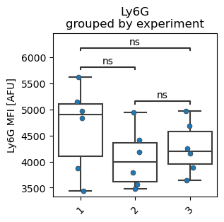
In order to visualize the data, we use the fp.pl.mfi() function. Similar to the previous fp.pl.cell_counts() and fp.pl.gate_frequency(), we use a categorical boxplot.
The gate parameter is used to specify the population. The default fp.settings.default_layer argument is compensated, so we access the previously calculated data on the compensated events.
[7]:
fp.pl.mfi(dataset,
          gate = "Neutrophils",
          groupby = "experiment",
          marker = "Ly6G")
No artists with labels found to put in legend. Note that artists whose label start with an underscore are ignored when legend() is called with no argument.
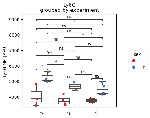
[8]:
fp.pl.mfi(dataset,
          gate = "Neutrophils",
          groupby = "experiment",
          splitby = "sex",
          stat_test = "Kruskal",
          marker = "Ly6G",
          figsize = (4,4))
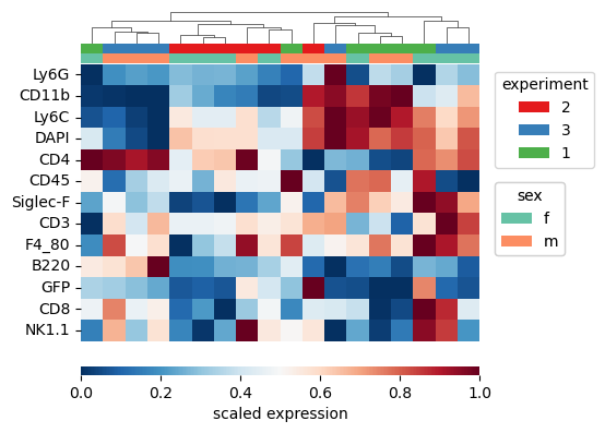
We can also plot the data as an expression heatmap. Here, we use the MFI values. Each row corresponds to a marker, and every column is a sample.
We use the metadata_annotation parameter in order to visualize the metadata on the same heatmap.
[9]:
fp.pl.expression_heatmap(dataset, gate = "CD45+", metadata_annotation = ["experiment", "sex"])
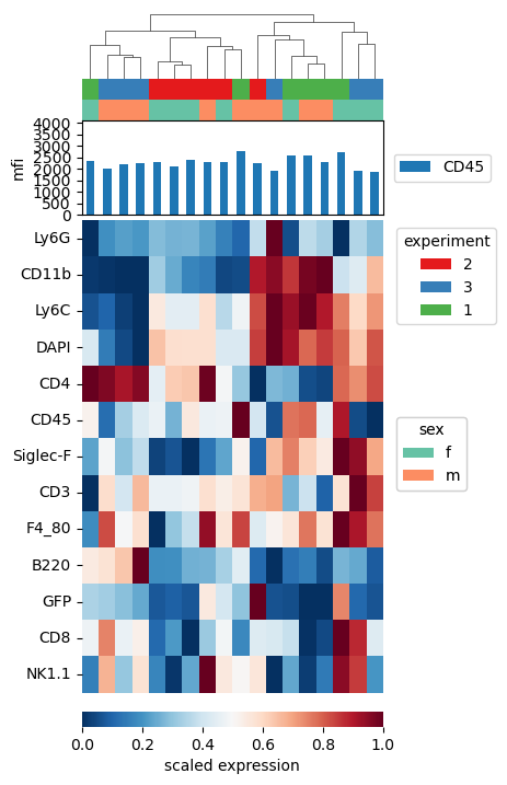
Often times, heatmaps can be misleading due to internal scaling. We can plot the raw MFI values for a specific marker on top by using the metadata_annotation parameter.
[10]:
fp.pl.expression_heatmap(dataset,
                         gate = "CD45+",
                         metadata_annotation = ["experiment", "sex"],
                         marker_annotation = "CD45",
                         figsize = (4,7))
FOP calculation#
In order to calculate the frequency of positives, a cutoff needs to be defined above which cells are counted as marker-positive.
In this example, we already performed the calculation of these cofactors, and these are stored in the .var slot.
[11]:
dataset.var
[11]:
| pns | png | pne | pnr | type | pnn | cofactors | |
|---|---|---|---|---|---|---|---|
| FSC-A | FSC-A | 1.0 | (0.0, 0.0) | 262144 | scatter | FSC-A | 1.0 |
| FSC-H | FSC-H | 1.0 | (0.0, 0.0) | 262144 | scatter | FSC-H | 1.0 |
| FSC-W | FSC-W | 1.0 | (0.0, 0.0) | 262144 | scatter | FSC-W | 1.0 |
| SSC-A | SSC-A | 1.0 | (0.0, 0.0) | 262144 | scatter | SSC-A | 1.0 |
| SSC-H | SSC-H | 1.0 | (0.0, 0.0) | 262144 | scatter | SSC-H | 1.0 |
| SSC-W | SSC-W | 1.0 | (0.0, 0.0) | 262144 | scatter | SSC-W | 1.0 |
| GFP | GFP | 1.0 | (0.0, 0.0) | 262144 | fluo | GFP-A | 604.5583 |
| B220 | B220 | 1.0 | (0.0, 0.0) | 262144 | fluo | APC-A | 621.9474 |
| CD4 | CD4 | 1.0 | (0.0, 0.0) | 262144 | fluo | APC-H7-A | 263.38608 |
| Siglec-F | Siglec-F | 1.0 | (0.0, 0.0) | 262144 | fluo | BV421-A | 5008.094 |
| CD8 | CD8 | 1.0 | (0.0, 0.0) | 262144 | fluo | BV510-A | 6000.0 |
| Ly6C | Ly6C | 1.0 | (0.0, 0.0) | 262144 | fluo | BV605-A | 566.7654 |
| NK1.1 | NK1.1 | 1.0 | (0.0, 0.0) | 262144 | fluo | BV711-A | 140.00124 |
| CD11b | CD11b | 1.0 | (0.0, 0.0) | 262144 | fluo | BV786-A | 495.22092 |
| Ly6G | Ly6G | 1.0 | (0.0, 0.0) | 262144 | fluo | BUV395-A | 127.525566 |
| DAPI | DAPI | 1.0 | (0.0, 0.0) | 262144 | fluo | BUV496-A | 1871.7664 |
| CD3 | CD3 | 1.0 | (0.0, 0.0) | 262144 | fluo | BUV737-A | 1767.76 |
| F4_80 | F4_80 | 1.0 | (0.0, 0.0) | 262144 | fluo | BYG790-A | 1105.7057 |
| CD45 | CD45 | 1.0 | (0.0, 0.0) | 262144 | fluo | BB700-A | 782.04565 |
| Time | Time | 1.0 | (0.0, 0.0) | 262144 | time | Time | 1.0 |
We can now calculate the frequency of parents using the fp.tl.fop() function. Similar to the MFI, FOPs are calculated per sample_ID and stored in the .uns slot.
[12]:
fp.tl.fop(dataset)
dataset
[12]:
AnnData object with n_obs × n_vars = 2450306 × 20
    obs: 'staining', 'sample_ID', 'file_name', 'organ', 'genotype', 'sex', 'experiment', 'age'
    var: 'pns', 'png', 'pne', 'pnr', 'type', 'pnn', 'cofactors'
    uns: 'metadata', 'panel', 'workspace', 'gating_cols', 'dataset_status_hash', 'cofactors', 'raw_cofactors', 'settings', 'pca_CD45+_transformed', 'pca_CD45+_logicle', 'gate_frequencies', 'mfi_sample_ID_compensated', 'fop_sample_ID_compensated'
    obsm: 'X_pca_CD45+_logicle', 'X_pca_CD45+_transformed', 'gating'
    varm: 'pca_CD45+_logicle', 'pca_CD45+_transformed'
    layers: 'compensated', 'logicle', 'transformed'
FOP visualization#
We use similar plotting capabilities for the display of FOPs.
[13]:
fp.pl.fop(dataset,
          marker = "Ly6G",
          gate = "CD45+",
          groupby = "experiment")
No artists with labels found to put in legend. Note that artists whose label start with an underscore are ignored when legend() is called with no argument.
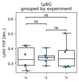
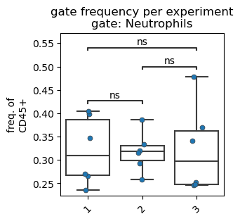
As Ly6G is a marker for Neutrophils, we expect the FOP to be very similar to the gate frequency of Neutrophils:
[14]:
fp.pl.gate_frequency(dataset,
                     gate = "Neutrophils",
                     freq_of = "CD45+",
                     groupby = "experiment")
No artists with labels found to put in legend. Note that artists whose label start with an underscore are ignored when legend() is called with no argument.
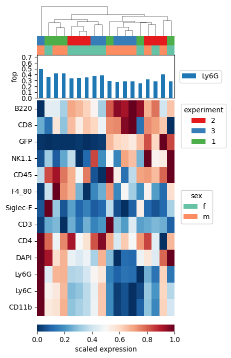
We can use the same expression heatmap as above, passing data_metric=fop. This will display the frequency of parents per sample as described above. Similarly, we display the frequency of Ly6G positive cells on top of the plot.
[15]:
fp.pl.expression_heatmap(dataset,
                         gate = "CD45+",
                         data_metric = "fop",
                         metadata_annotation = ["experiment", "sex"],
                         marker_annotation = "Ly6G",
                         figsize = (4,7))
Save the dataset#
Since we performed the mfi and fop analysis, we save the dataset.
[16]:
fp.save_dataset(dataset,
                file_name = "../../Tutorials/mouse_lineages/raw_dataset_stained_mfi",
                overwrite = True)
File saved successfully